导包

#conding=utf-8
import pandas as pd
import numpy as np
import matplotlib.pyplot as plt

from sklearn.linear_model import LinearRegression
from mpl_toolkits.mplot3d import axes3d

# pandas 基础设置
pd.set_option('display.notebook_repr_html',False)
pd.set_option('display.max_columns',None)
pd.set_option('display.max_rows',150)
pd.set_option('display.max.seq_items',None)

%matplotlib inline

import seaborn as sns  # 格式化工具
sns.set_context('notebook')
sns.set_style('white')

定义方法

# n阶单位阵
def warmUpExercise(n):
    return(np.identity(n))

损失函数

# 计算损失函数
def computeCost(X, y, theta=[[0], [0]]):
    m = y.size  # 总样本点
    J = 0

    h = X.dot(theta)  # 向量点积和矩阵乘法

    J = 1.0 / (2 * m) * (np.sum(np.square(h - y)))  # cost function

    return J

梯度下降

# 梯度下降
#  alpha:学习率  num_iters:迭代轮次   
def gradientDescent(X, y, theta=[[0], [0]], alpha=0.01, num_iters=150):
    m = y.size
    J_history = np.zeros(num_iters)

    for iter in np.arange(num_iters):
        h = X.dot(theta)  # 函数
        theta = theta - alpha * (1.0 / m) * (X.T.dot(h - y))  # 一元的损失函数
        J_history[iter] = computeCost(X, y, theta)  # 每次迭代后计算的损失函数
    return (theta, J_history)

引入数据

# txt的数据格式如下：
# 5,800
# 10,1000
# 15,1500
# 20,2000
data = np.loadtxt('linear_regression_data1.txt',delimiter=',')
X = np.c_[np.ones(data.shape[0]),data[:,0]]  # np.c_是按行连接两个矩阵   X:样本点
y = np.c_[data[:,1]]  # y：结果点

画图

# x,y：输入数据  s:标量  c:颜色  marker:标记   linewidths：线宽
plt.scatter(X[:,1], y, s=30, c='r', marker='x', linewidths=1)  # 散点图
plt.xlim(4,24)  # x轴边界  取值范围
plt.xlabel('Population of City in 10,000s')  # x 人口
plt.ylabel('Profit  in $10,000s')  # y 收益
# plt.show()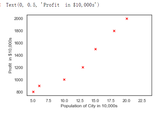

# 画出每一次迭代和损失函数变化
theta , Cost_J = gradientDescent(X, y)
print('theta: ',theta.ravel())  # .ravel()将多维数组降位一维

plt.plot(Cost_J)
plt.ylabel('Cost J')
plt.xlabel('Iterations');
# plt.show()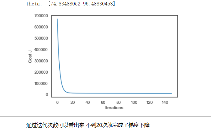

xx = np.arange(5,23)  # 函数返回一个有终点和起点的固定步长的排列
yy = theta[0]+theta[1]*xx

# 画出我们自己写的线性回归梯度下降收敛的情况
plt.scatter(X[:,1], y, s=30, c='r', marker='x', linewidths=1)
plt.plot(xx,yy, label='Linear regression (Gradient descent)')  # 画线

# 和Scikit-learn中的线性回归对比一下
regr = LinearRegression()  # 线性回归方法
regr.fit(X[:,1].reshape(-1,1), y.ravel())  #  放入X  y的参数
plt.plot(xx, regr.intercept_+regr.coef_*xx, label='Linear regression (Scikit-learn GLM)')  # 画线

plt.xlim(4,24)
plt.xlabel('Population of City in 10,000s')
plt.ylabel('Profit in $10,000s')
plt.legend(loc=4)  # 函数主要的作用就是给图加上图例
plt.show()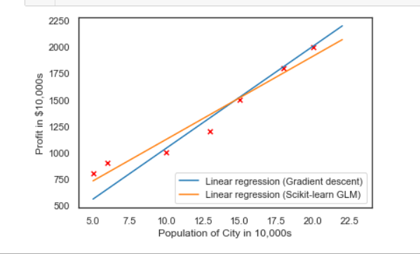

预测

# 预测一下人口为35000和70000的城市的结果
print(theta.T.dot([1, 3.5])*10000)
print(theta.T.dot([1, 7])*10000)

[4125439.46381248] [7502530.12246606]